In this blog post I’ll explain this advection algorithm and how to use it to make advanced fluid simulations like the ones I made, including Paint streams and Everflow. Before starting, I should give a big thanks to my friend Wyatt for giving useful suggestions on building this algorithm.

Looks really smooth, doesn’t it? It even captures droplets with almost close to pixel level precision. And while it does model a fluid with a boundary it does not use particles directly like in SPH, but is actually a semi-Lagrangian grid based algorithm. Oh, and I forgot to say - it’s also super fast.

Let’s start with a brief history, the initial idea for this algorithm came from trying to extend screen space voronoi particle tracking to avoid particle loss, indeed when trying to store the particle state in screen space as close to the particle location as we can, in the case of overlap one of the particles will be lost, and there is no way to avoid it. But actually we can reformulate the problem, what if we don’t try to avoid particle overlap but tried to conserve the total mass? Like by adding the overlapping particle masses together and weighting their velocities and positions by mass. Actually that was already tried by stb, but it immediately becomes apparent that the total number of particles drops proportionally to the particle/pixel density because of them combining, you might ask if there is a way to separate them back, or if there is a way to achieve approximate particle number conservation? In fact, it is possible, but let’s overview how he does the particle tracking first.

Cellular automaton particle tracking

This algorithm is similar to a lattice gas automaton where the state of each cell is defined by a few discrete levels, is the particle in the cell and in which discrete direction it is moving. In our case instead of using a few discrete states we store the position, velocity and mass of the particle within the cell as floats (or any other number type, depends on the precision you want to achieve, I actually used 2 int16’s per channel since Shadertoy only has a 4 channel output per pixel and I needed to store at least 5 numbers)

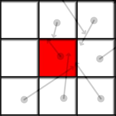
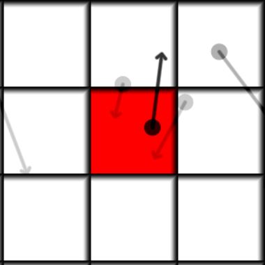
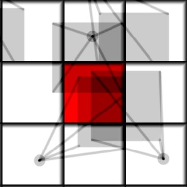
Initial Frame	Next frame

The main idea of the algorithm is to loop over all neighbors of the current cell(including itself), integrate the position of each neighbor particle and add it if it ends up in this cell. Above is a visualization of how it looks like. Each cell has a particle with a mass, the mass is shown by opacity, so 0 mass is invisible and 1 is completely dark. The red cell is our current cell for which we want to find its future state, the future position of the particles is shown by the arrow. We can see that there is more than one particle moving into the red cell. So in the end all the particles that end up in the same cell are summed and their positions and velocities are averaged. In mathematical form it can be written as:

\[ M_{i}^{t+1} = \sum_{j}^\textrm{neighbors} K_{i}(\vec{X}_ {j}^{t} + \Delta t \vec{V}_ {j}^{t}) m_{j}^{t} — \textrm{updated mass} \] \[ \vec{X}_ {i}^{t+1} = \frac{1}{M_ {i}^{t+1}} \sum_{j}^\textrm{neighbors} K_{i}(\vec{X}_ {j}^{t} + \Delta t \vec{V}_ {j}^{t}) (\vec{X}_ {j}^{t} + \Delta t \vec{V}_ {j}^{t}) m_{j}^{t} — \textrm{updated center of mass} \] \[ \vec{V}_ {i}^{t+1} = \frac{1}{M_ {i}^{t+1}} \sum_{j}^\textrm{neighbors} K_{i}(\vec{X}_ {j}^{t} + \Delta t \vec{V}_ {j}^{t}) \vec{V}_ {j}^{t} m_{j}^{t} — \textrm{updated velocity} \] Where \(M_{i}^{t}\) is the mass of the particle in cell i on time step t, \(\vec{X}_ {i}^{t}\) is the position of the particle and \(\vec{V}_ {i}^{t}\) is the velocity. The function \(K_{i}(\vec{X})\) is equal to 1 if the point \(\vec{X}\) is inside the cell i, and zero otherwise. \( \Delta t \) is the timestep.

For a square cell the K function is simply \[ K_{i}(\vec{X}) = H(\vec{X} - \vec{C}_ {i} + 0.5) H(\vec{C}_ {i} + 0.5 - \vec{X}) \] Where \(H\) is the multivariate Heaviside step function. \(\vec{C}_{i}\) is the center of cell i.

It’s quite a simple algorithm, but it has one limitation, to ensure that we counted every possible particle that might end up in this cell we would either need to loop over the entire grid, which is highly expensive, or limit the maximum velocity of the particles to make the search radius finite, and hopefully only 1 pixel wide.

Obviously the second option is much better in our context, and in fact if we want to track particles with velocities so fast that they traverse the grid in 1 frame it’s actually cheaper to do lots of smaller steps with a 1 pixel neighborhood instead of counting all cells in one step, since \( 9 \sqrt{N} < N \) , where N is the number of cells, and the square root is because we need to apply the operation only a linear amount of times, instead of applying it for every cell. And the 9 is the number of neighbors. In 3D it would equivalently be \( 27 N^{1/3} < N \) which is even more efficient. I should note that more steps does not mean better quality, since the particles may combine together on the way. Also we can just do the tracking on CPU, and do it in a forward way, just loop over all particles and add them into the right cells, then we would not care about those things, but we obviously want to use that GPU power to our advantage.

Here is a pseudo-code glsl implementation of this algorithm:

//this cell position
ivec2 pos;
//values stored in the cell
vec2 velocity = vec2(0.), position = vec2(0.);
float mass = 0.;
//find and average the particles 
//that land in this cell after a time step dt
for(int x = -R; x <= R; x++) //only check the neighbors at radius R
  for(int y = -R; y <= R; y++)
  {
      //get the particle in this neighbor cell from the previous frame
      particle P = getParticle(pos + ivec2(x,y));
      //integrate the particle position
      P.X += P.V*dt;
      //check if the particle is inside of this cell
      if(inCell(P, pos))
      {
        mass += P.M; //add the particle mass to this cell
        position += P.X*P.M; //add the particle position weighted by mass
        velocity += P.V*P.M; //add the particle velocity weighted by mass(momentum)
      }
  } 

//normalize
if(mass > 0.0) //if not vacuum
{
  position /= mass; //center of mass
  velocity /= mass; //average velocity
}

Dividing particles

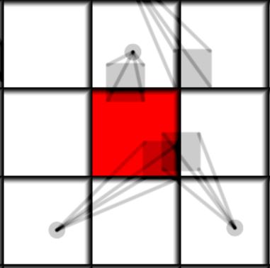
To combat the problem of a decreasing particle number we can try and divide each particle into M virtual particles with distributed positions that might end up in different cells and thus increase the total number of particles.

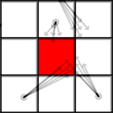
The radius of the distribution defines how likely is the particle is to multiply. If the all the virtual particles end up inside of a single cell the particle would not divide and stay essentially the same(if the average particle of the virtual particles is equal to the original particle). To make it properly conservative we just need to divide the mass of the particle into a number of equal chunks, and make sure the distribution average is zero.

On the picture above and in the code below we see an example for a 5 virtual particle distribution, the average of the distribution directions is zero and its radius is 0.1 pixels.

Here is the code, the only addition are the diffusion directions and a loop for each of the virtual particles.

//this cell position
ivec2 pos;
//values stored in the cell
vec2 velocity = vec2(0.), position = vec2(0.);
float mass = 0.;

//diffusion radius
float difR = 0.1;
//diffusion directions
vec2 difDir[5] = {vec2(0,0),vec2(1,0),vec2(-1,0),vec2(0,1),vec2(0,-1)};

//find and average the particles 
//that land in this cell after a time step dt
for(int x = -R; x <= R; x++) //only check the neighbors at radius R
  for(int y = -R; y <= R; y++)
  {
      //get the particle in this neighbor cell from the previous frame
      particle P = getParticle(pos + ivec2(x,y));
      //integrate the particle position
      P.X += P.V*dt;
      for(int i = 0; i < 5; i++) //divide particle into 5
      {
        particle difP = P;
        difP.X += difR*difDir[i]; //move particle in one of the diffusion directions
        difP.M /= 5.0; //divide mass into 5 particles

        //check if the divided particle is inside of this cell
        if(inCell(difP, pos))
        {
          mass += difP.M; //add the particle mass to this cell
          position += difP.X*difP.M; //add the particle position weighted by mass
          velocity += difP.V*difP.M; //add the particle velocity weighted by mass(momentum)
        }
      }
  } 

//normalize
if(mass > 0.0) //if not vacuum
{
  position /= mass; //center of mass
  velocity /= mass; //average velocity
}

You might ask if its possible to achieve a perfect particle number conservation, and not just total mass conservation. Actually to do that we just need to divide the mass into integer chunks that sum into the original mass, the virtual particles need not be the same, so for example one particle with mass 3 can divide into 2 particles with mass 2 and 1. Dividing into more than 2 virtual particles is pretty much the same, even though a bit more complicated.

Using particle distributions

The previous algorithm did solve the problem sufficiently well, but did have some shortcomings, like the additional loop which makes that algorithm far slower to execute and produces discontinuities in density that made it harder to implement fluid simulations. We can actually do better. Lets look at the limiting case of an infinite number of virtual particles, in such a case we end up with a continuous distribution of mass that we can call \( \rho(\vec{X}) \) (the distribution should also be centered on the particle position).

So to find the amount of mass (and its center) each particle deposits into this cell we need to integrate the distribution within the current cell bounds. (And that is where I got the name - reintegrating tracked particle distributions) Our equations are: \[ M = \int \int_{\Omega} \rho(\vec{X})d\vec{X} — \textrm{deposited mass} \] \[ \vec{C} = \frac{1}{M} \int \int_{\Omega} \vec{X}\rho(\vec{X})d\vec{X} — \textrm{deposited center of mass} \] Where \( \Omega \) is the cell region. But which distribution should we use? If we try to use a normal distribution we will end up with the problem of how to compute it, since there is no analytical solution for such an integral, and we would need to numerically integrate the distribution, which is not much better performance-wise than the previous algorithm. The simplest distribution that gives an analytical solution we can use is actually a uniform axis aligned box, for which the mass and the center of mass are trivial to compute analytically. We can also try a uniform circular distribution or a nonuniform circular distribution equal to \( 1 - |\vec{X_0} - \vec{X}|^2 \) for \( |\vec{X_0} - \vec{X}| \leqslant 1\) and equal to \( 0 \) for \( |\vec{X_0} - \vec{X}| > 1 \) where \( \vec{X_0} \) is the particle position, but let’s try out the simplest approach.

Diffusion radius 0.2	Diffusion radius 0.55

To find the mass and center of mass of the distribution within the bounds of the cell we only need to figure out the overlap box of the cell and the particle distribution. Its relative area will be the relative mass and its center is just the center of mass. It can be implemented like this:

//this cell position
ivec2 pos;
//values stored in the cell
vec2 velocity = vec2(0.), position = vec2(0.);
float mass = 0.;
//find and average the particles 
//that land in this cell after a time step dt
for(int x = -R; x <= R; x++) //only check the neighbors at radius R
  for(int y = -R; y <= R; y++)
  {
      //get the particle in this neighbor cell from the previous frame
      particle P = getParticle(pos + ivec2(x,y));
      //integrate the particle position
      P.X += P.V*dt;
      //find the overlap of the diffused particle distribution with this cell
      
      vec3 ovrlp = overlap(P.X, pos, diffusion_radius);
      float overlapRelativeArea = ovrlp.z;
      vec2 overlapCenterOfMass = ovrlp.xy;
      float overlapMass = overlapRelativeArea*P.M;

      mass += overlapMass; //add the overlap mass to this cell
      position += overlapCenterOfMass*overlapMass; //add the overlap center weighted by mass
      velocity += P.V*overlapMass; //add the particle velocity weighted by overlap mass(momentum)
  } 

//normalize
if(mass > 0.0) //if not vacuum
{
  position /= mass; //center of mass
  velocity /= mass; //average velocity
}

The axis alligned box overlap calculation is rather straightforward

vec3 overlap(vec2 x, vec2 p, float diffusion_radius)
{
    vec4 aabb0 = vec4(p - 0.5, p + 0.5); //cell box
    vec4 aabb1 = vec4(x - diffusion_radius, x + diffusion_radius); //particle box
    vec4 aabbX = vec4(max(aabb0.xy, aabb1.xy), min(aabb0.zw, aabb1.zw)); //overlap box
    vec2 center = 0.5*(aabbX.xy + aabbX.zw); //center of mass 
    vec2 size = max(aabbX.zw - aabbX.xy, 0.); //only positive
    float m = size.x*size.y/(4.0*diffusion_radius*diffusion_radius); //relative area
    //if any of the dimensions are 0 then the mass ratio is 0
    return vec3(center, m);
}

As you can see we don’t need to loop over virtual particles anymore since the solution is analytical, so the performance of this approach is the same as in the original cellular automaton particle tracker with the added benefit of giving much smoother results.

And here is a real time visualization of the reintegration process with diffusion radius 0.35

In fact this algorithm has some quite interesting properties, depending on the radius of the distribution the behaviour can change from particle-like to field-like as shown in the simulation below(you need to unpause it). The distribution diameter oscillates between 0.75 and 1.25:

We can see that for a diameter less than 1 pixel the behaviour tends to be particle-like and for a larger one it behaves more like usual advection with numerical diffusion.

Another interesting fact is that if we fix the particle positions to the cell centers and set the distribution radius to 0.5 so that the distribution is exactly as big as the cell we’ll get exactly forward Euler advection! Since we are technically just integrating the cells forward and depositing their contents.

Using the SPH formulation instead of finite differences to compute forces

Now what are we going to do with this algorithm? We can use the grid and compute finite difference gradients to compute forces. But we are actually losing the sub-cell distribution information - the cell centers of mass.

Since it can model particle systems we can try to adapt particle algorithms here, for example molecular dynamics(it would need exact particle count conservation), or maybe how about using smoothed particle hydrodynamics(SPH)? Actually this algorithm gives pretty much the perfect conditions for SPH, the particles are already uniformly distributed, around 1 particle per cell, and we can quite easily find the particle neighbors, since the grid itself is an acceleration structure! And that is pretty much exactly what was done in Paint streams or Everflow. With a large enough distribution radius (0.55-0.6) the natural diffusion is smoothing the particles so that we get away with a relatively small smoothing kernel, about 1.5 pixels wide, and we only need to compute the forces from the closest neighbors which makes it even more efficient.

To implement SPH we just need to integrate the new cell velocity using the reintegrated particle distributions.

\[ \vec{V}_ {i}^{t+1} = \vec{V}_ {i}^{t} +\Delta t \frac{\vec{F}_ {i}}{M_ {i}^{t}} — \textrm{updated velocity} \] Where \(\vec{F}_ {j}\) is the computed SPH force [1] computed for the particle in cell i.

\[ \vec{F}_ {i} =M_ {i}^{t} \sum_{j}^\textrm{neighbors} M_ {j}^{t} \left( \frac{P_{i}}{\rho_{i}^2} + \frac{P_{j}}{\rho_{j}^2} \right) \nabla_{i} W(\vec{X}_ {j}^{t} - \vec{X}_ {i}^{t}) \]

Where \(P_{i}\) is the pressure in cell i, and \(W(\vec{X})\) is the smoothing kernel. For the density \( \rho_{i} \) we can just use the mass of the cell divided by its volume, assuming the volume is 1 we can just place the mass. It’s ok to do so if the the distribution radius is big enough to smooth out the mass.

Pressure for each cell can just be computed using an equation of state. For a gas its simply just proportional to the cell density times the temperature, but let’s consider only constant temperatures:

\[ P_{i} = k \rho_{i} \] Where k is some proportionality constant.

For a fluid we can use the Cole equation of state \[ P_{i} = k \left( \left(\frac{\rho_{i}}{\rho_{0}} \right)^ \gamma - 1 \right) \]

Where \(\gamma\) is the adiabatic index (\(\gamma = 7.0\) for water), \(\rho_{0}\) is the reference fluid density.

In most of my simulations I just used the following pressure, which worked quite well in this setting. \[ P_{i} = k \rho_{i} (\rho_{i} - \rho_{0}) \]

Storing more properties inside a cell

There is nothing holding us from storing a more advanced description of the insides of the cell, we can store not just a particle - but an entire distribution, and we can also update its size depending on the variations of the centers of mass of other distributions that fell into this cell. We can also store the angular momentum of such a distribution to preserve vorticity in fluids for example, sadly averaging angular momentums of distribution parts is a bit complicated, and my experiments are not entirely stable and require angular momentum clamping suggesting that the way I added them was not exact (the colors show the curl value in the fluid). If I happen to successfully implement such a summation I will write a follow-up article, since perfect angular momentum tracking is really important for nice vortices.

Conclusions

This is a really cool algorithm, and I wanted to share it with other people the moment I had the first successful results, Wyatt has already used it for some really cool simulations, including multi-substance interactions. Thanks to the mass conserving quality of the advection it can be used to model self-gravitating gas too (the angular momentum there is total whack tho, but looks cool)

Other interesting use cases are:

• Modelling boilling - very approximately, the equation of state is not that good there.
• Fluid advection with a pressure computed using the Poisson equation.
• Rocket Mach diamonds - modelling supersonic gas using a gas equation of state.
• Slime molds - I should probably make a blog post on this too.
• Life-like cells - ????. Another post needed, yeah.

Also here is a processing implementation of reintegration tracking (no SPH forces)

References

[1] Smoothed Particle Hydrodynamics